Examples

These examples use finance-datagen for deterministic market-like inputs and finance-calcs for returns and technical indicators. The plotting functions then consume ordinary pandas Series, Polars Series, or numpy arrays.

---

Shared Setup

from datetime import date, datetime, timezone

import pandas as pd
import polars as pl
from finance_datagen import generate_prices, generate_signal

import finance_calcs as fc
import finance_plots as fp


def as_series(frame: pl.DataFrame, column: str, *, drop_nulls: bool = False) -> pd.Series:
    data = frame.select("timestamp", column)
    if drop_nulls:
        data = data.drop_nulls()
    return pd.Series(
        data[column].to_numpy(),
        index=data["timestamp"].to_pandas(),
        name=column,
    )


start_ms = int(datetime(2021, 1, 4, tzinfo=timezone.utc).timestamp() * 1000)
prices = generate_prices(n_steps=756, symbol="ACME", seed=7, start_ms=start_ms)
benchmark_prices = generate_prices(
    n_steps=756,
    symbol="BENCH",
    seed=11,
    start_ms=start_ms,
    mu=0.04,
    sigma=0.16,
)

price_frame = prices.with_columns(
    fc.simple_returns(pl.col("price")).alias("ret"),
    fc.sma(pl.col("price"), window=20).alias("sma20"),
    fc.ema(pl.col("price"), window=60).alias("ema60"),
    fc.rsi(pl.col("price"), window=14).alias("rsi14"),
    fc.macd_line(pl.col("price")).alias("macd"),
    fc.macd_signal(pl.col("price")).alias("macd_signal"),
)
benchmark_frame = benchmark_prices.with_columns(
    fc.simple_returns(pl.col("price")).alias("ret"),
)

returns = as_series(price_frame, "ret", drop_nulls=True)
benchmark = as_series(benchmark_frame, "ret", drop_nulls=True)
price = as_series(price_frame, "price")
sma20 = as_series(price_frame, "sma20")
ema60 = as_series(price_frame, "ema60")
rsi14 = as_series(price_frame, "rsi14")
macd = as_series(price_frame, "macd")
macd_signal = as_series(price_frame, "macd_signal")

trade_transactions = pl.DataFrame(
    {
        "timestamp": [date(2021, 1, 4), date(2021, 1, 6), date(2021, 1, 8), date(2021, 1, 11), date(2021, 1, 13)],
        "symbol": ["ACME", "ACME", "ACME", "BETA", "BETA"],
        "amount": [100.0, -40.0, -60.0, -80.0, 80.0],
        "price": [100.0, 106.0, 96.0, 50.0, 44.0],
        "commission": [1.0, 1.0, 1.0, 1.0, 1.0],
        "fees": [0.25, 0.25, 0.25, 0.25, 0.25],
        "bps": [4.0, 6.0, 5.0, 7.0, 4.0],
    }
)
cost_breakdown = fc.cost_attribution(trade_transactions)
round_trips = fc.extract_round_trips(trade_transactions)
excursion_prices = pl.DataFrame(
    {
        "timestamp": [date(2021, 1, 4), date(2021, 1, 5), date(2021, 1, 6), date(2021, 1, 7), date(2021, 1, 8)] * 2,
        "symbol": ["ACME"] * 5 + ["BETA"] * 5,
        "price": [100.0, 94.0, 106.0, 112.0, 96.0, 50.0, 53.0, 47.0, 43.0, 44.0],
    }
)
trades_with_excursions = fc.mae_mfe(round_trips, excursion_prices)
execution_quality = pd.DataFrame(
    {
        "timestamp": pd.date_range("2021-01-04", periods=12, freq="B"),
        "implementation_shortfall_bps": [9.0, 12.0, -3.0, 6.0, 15.0, 4.0, 8.0, -2.0, 11.0, 7.0, 5.0, 13.0],
    }
)

signals = generate_signal(n_dates=80, n_assets=40, ic=0.12, seed=23, start=date(2021, 1, 4)).with_columns(
    pl.when(pl.col("symbol").str.slice(-1).is_in(["0", "2", "4", "6", "8"]))
    .then(pl.lit("Tech"))
    .otherwise(pl.lit("Energy"))
    .alias("group")
)
signals = signals.with_columns(fc.assign_quantile(pl.col("signal"), 5).over("date").alias("quantile"))
ic_frame = signals.group_by("date").agg(fc.information_coefficient_spearman(pl.col("signal"), pl.col("fwd_returns")).alias("ic")).sort("date")
ic_by_group = signals.group_by("date", "group").agg(fc.information_coefficient_spearman(pl.col("signal"), pl.col("fwd_returns")).alias("ic")).sort("date")
changed = signals.sort("symbol", "date").with_columns(fc.quantile_changed(pl.col("quantile")).over("symbol").alias("changed"))
turnover = changed.group_by("date", "quantile").agg(fc.quantile_turnover(pl.col("changed")).alias("turnover"))
quantile_returns = signals.group_by("date", "quantile").agg(
    pl.col("fwd_returns").mean().alias("return"),
    pl.len().alias("count"),
    pl.col("signal").mean().alias("signal_mean"),
)
alpha_frame = quantile_returns.join(turnover, on=["date", "quantile"], how="left").sort("date", "quantile").to_pandas()
factor_returns_frame = signals.group_by("date").agg(
    fc.long_short_spread(pl.col("fwd_returns"), pl.col("quantile"), upper=4, lower=0).alias("factor_return")
).sort("date")
ic = pd.Series(ic_frame["ic"].to_numpy(), index=ic_frame["date"].to_pandas(), name="ic")
factor_returns = pd.Series(
    factor_returns_frame["factor_return"].to_numpy(),
    index=factor_returns_frame["date"].to_pandas(),
    name="factor_return",
)

---

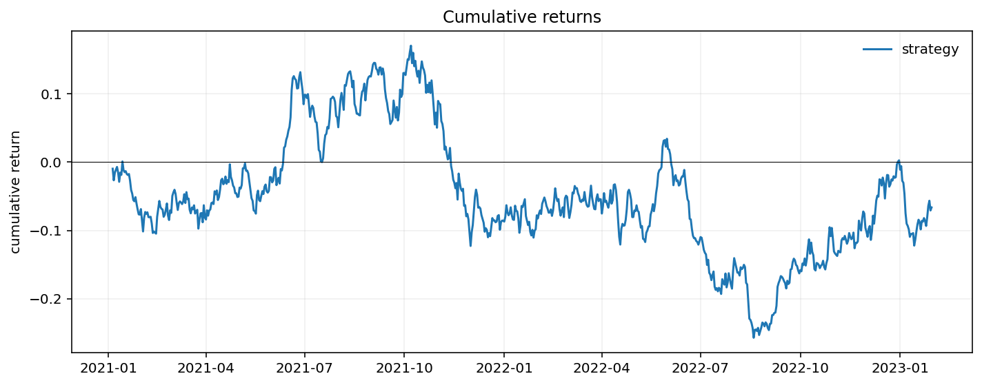
Return Path

fig = fp.plot_returns(returns)

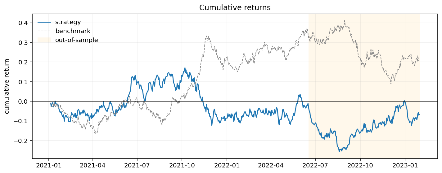
Return Path With Benchmark

fig = fp.plot_rolling_returns(
    returns,
    benchmark=benchmark,
    live_start=returns.index[int(len(returns) * 0.7)],
)

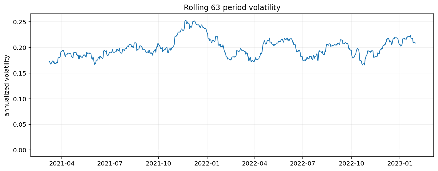
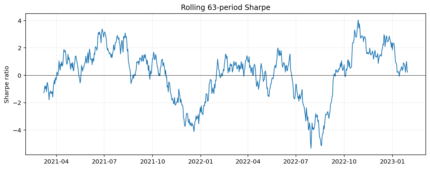
Rolling Volatility, Sharpe, and Beta

vol_fig = fp.plot_rolling_volatility(returns, window=63)
sharpe_fig = fp.plot_rolling_sharpe(returns, window=63)
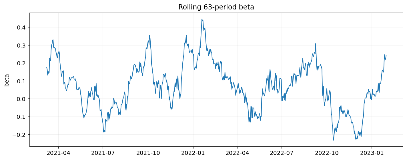
beta_fig = fp.plot_rolling_beta(returns, benchmark, window=63)

Benchmark Relationship

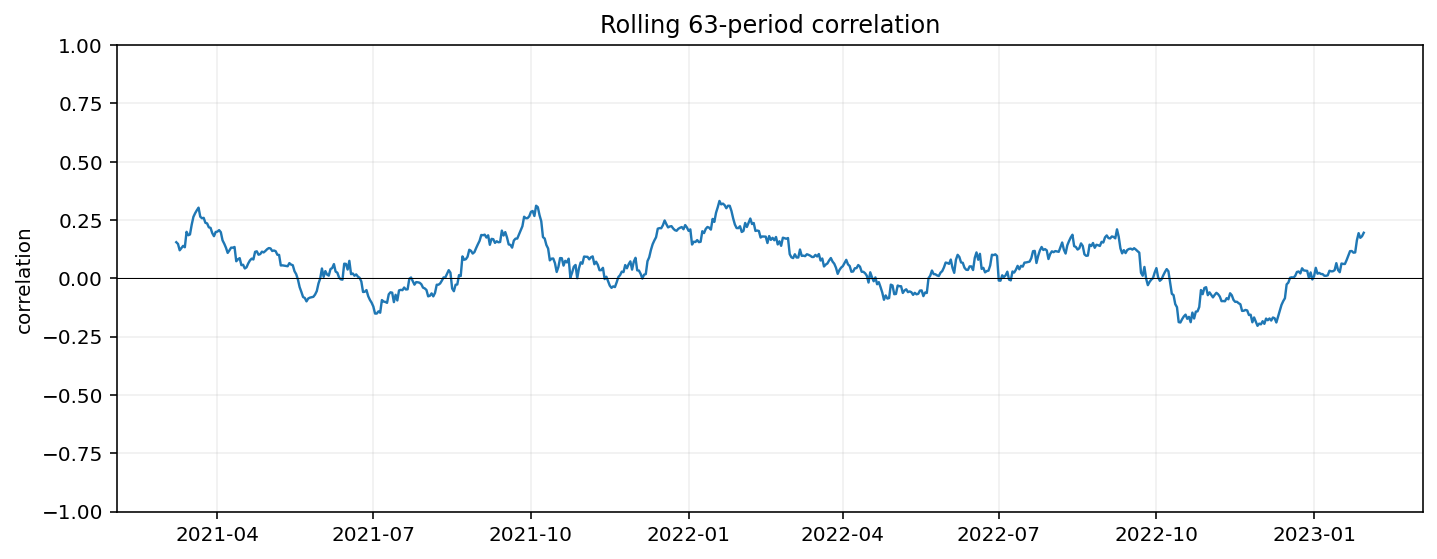
corr_fig = fp.plot_rolling_correlation(returns, benchmark, window=63)
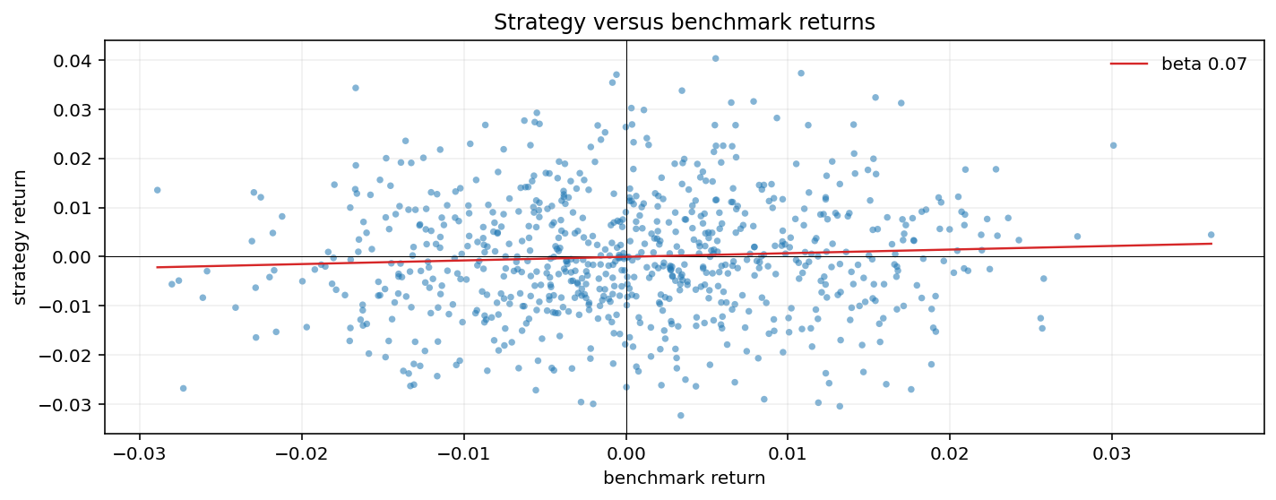
scatter_fig = fp.plot_return_scatter(returns, benchmark)

Drawdown

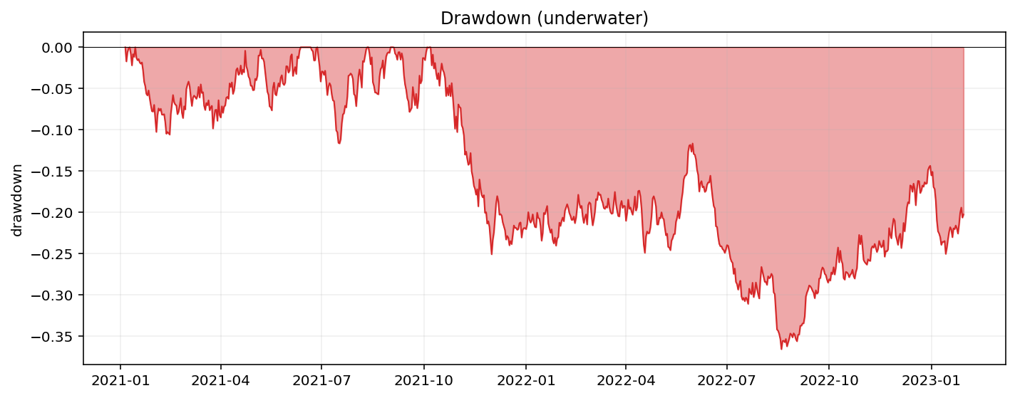
fig = fp.plot_drawdown_underwater(returns)

Return Heatmap

fig = fp.plot_returns_heatmap(returns, period="month")

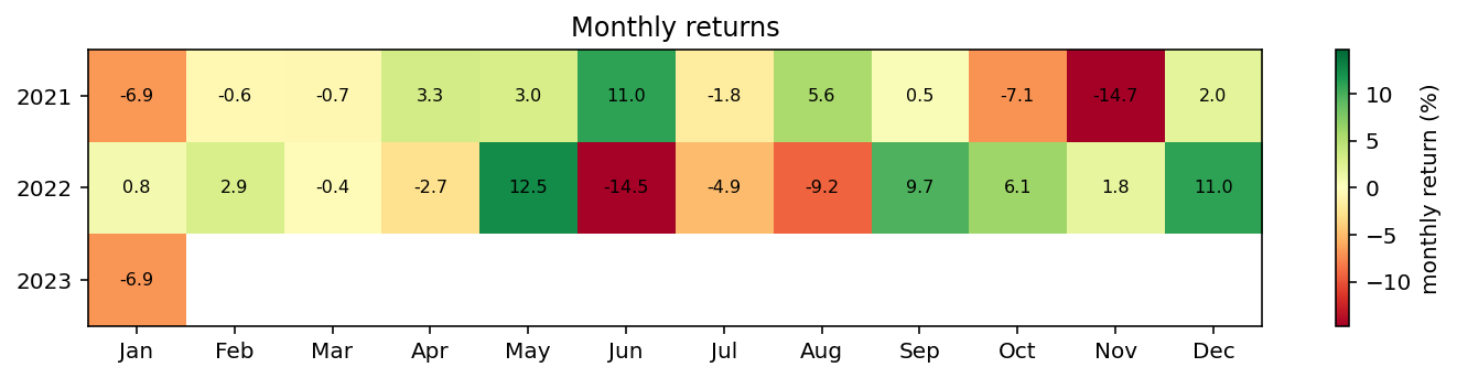
Quarterly and weekly buckets use the same function:

quarterly_fig = fp.plot_returns_heatmap(returns, period="quarter")
weekly_fig = fp.plot_returns_heatmap(returns, period="week")

Period Return Bar, Distribution, and Timeseries

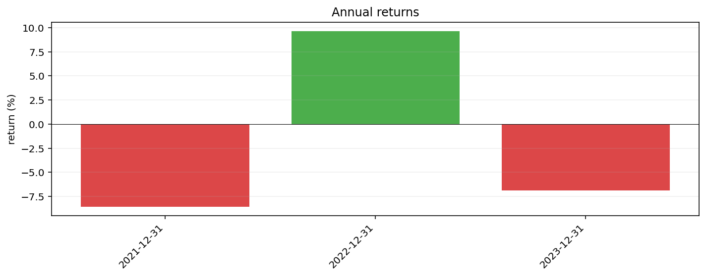
annual_bar = fp.plot_returns_bar(returns, period="year")
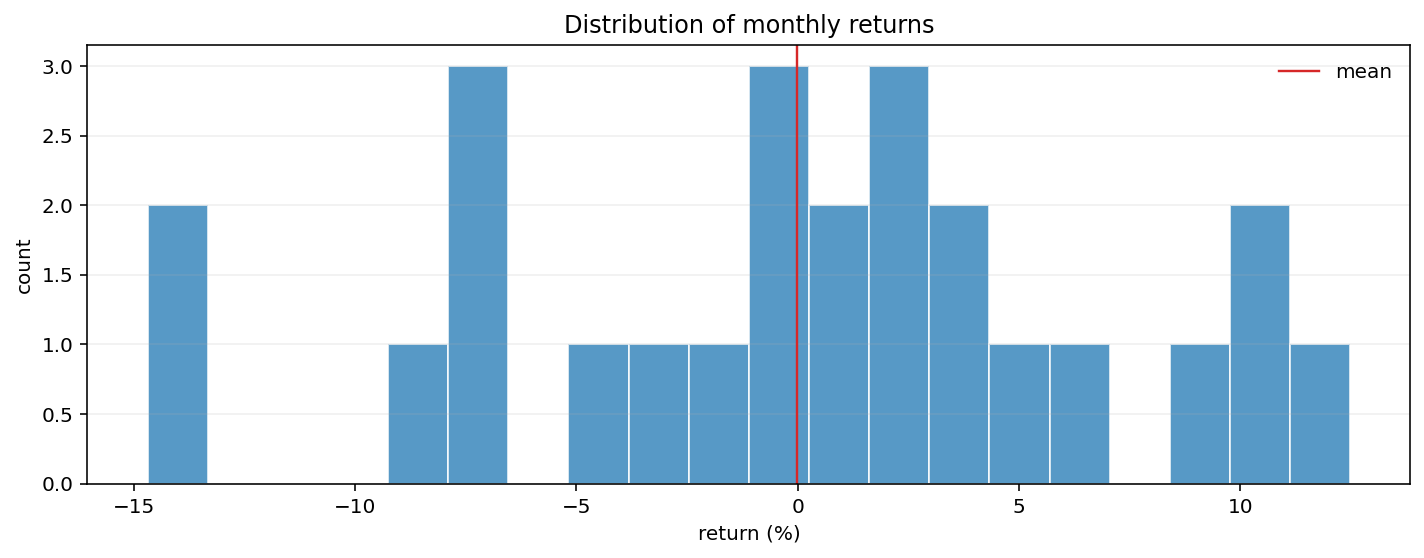
monthly_dist = fp.plot_returns_dist(returns, period="month")
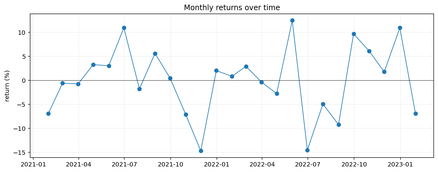
monthly_series = fp.plot_returns_timeseries(returns, period="month")

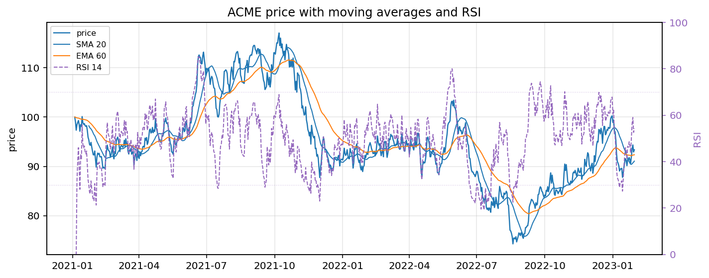
Price Overlays

fig = fp.plot_price_with_overlays(
    price,
    overlays=[("SMA 20", sma20), ("EMA 60", ema60)],
    secondary_overlays=[("RSI 14", rsi14)],
    secondary_ylabel="RSI",
    title="ACME price with moving averages and RSI",
)

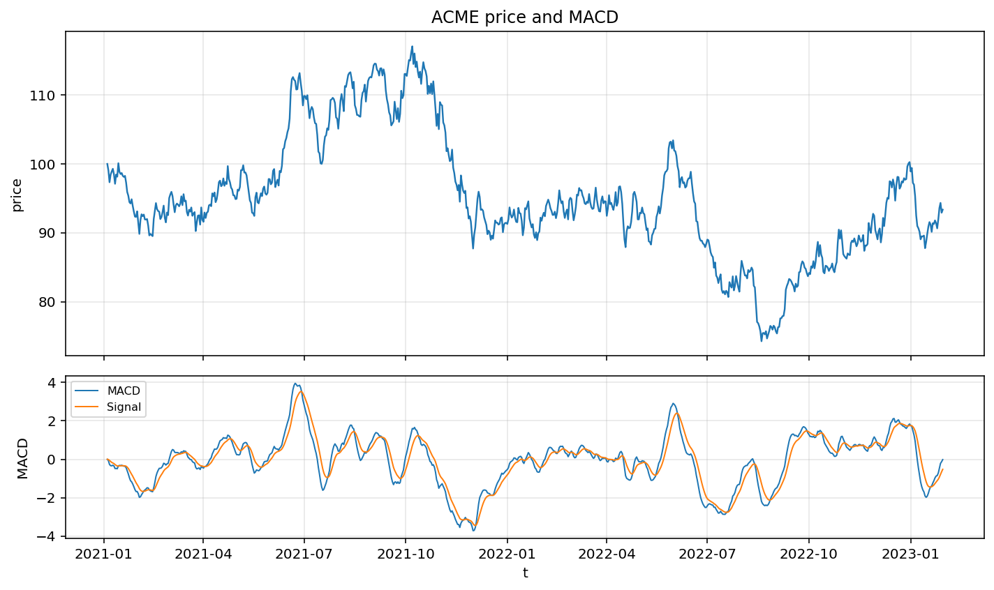
Indicator Panels

fig = fp.plot_indicator_panel(
    price,
    panels=[{"title": "MACD", "series": [("MACD", macd), ("Signal", macd_signal)]}],
    title="ACME price and MACD",
)

Performance Statistics

stats = fp.performance_statistics(returns)

Metric	Value
Cumulative return	-6.64%
Annualized return	-2.26%
Annualized volatility	19.82%
Sharpe ratio	-0.02
Sortino ratio	-0.02
Max drawdown	-36.56%
Calmar ratio	-0.06

Performance Table

table = fp.table_performance_statistics(returns, benchmark=benchmark)
html = table.as_raw_html()

Metric	Strategy	Benchmark
Cumulative return	-6.64%	21.19%
Annualized return	-2.26%	6.62%
Annualized volatility	19.82%	16.68%
Sharpe ratio	-0.02	0.47
Sortino ratio	-0.02	0.68
Max drawdown	-36.56%	-22.92%
Calmar ratio	-0.06	0.29

table_performance_statistics.html

Period Return Table

period_table = fp.table_period_returns(returns, period="year")

Period	Return
2021	-8.56%
2022	9.66%
2023	-6.89%

Drawdown Table

drawdown_table = fp.table_drawdowns(returns, top=5)

Rank	Start	Trough	Recovery	Drawdown	Duration
1	2021-10-07	2022-08-19	Unrecovered	-36.56%	480
2	2021-06-27	2021-07-17	2021-08-11	-11.64%	45
3	2021-01-14	2021-02-14	2021-06-12	-10.57%	149
4	2021-09-03	2021-09-18	2021-10-04	-7.83%	31
5	2021-08-12	2021-08-21	2021-09-01	-5.70%	20

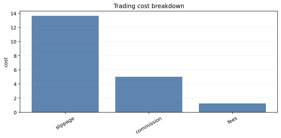
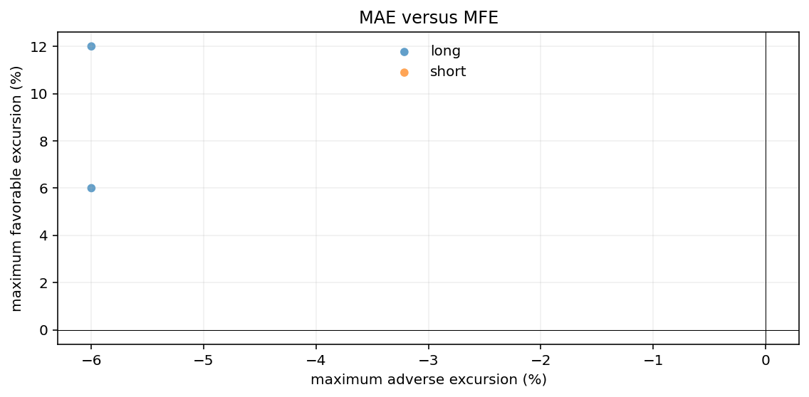
Post-Trade Plots

cost_fig = fp.plot_trading_cost_breakdown_bar(cost_breakdown)
mae_mfe_fig = fp.plot_mfe_mae_scatter(trades_with_excursions)
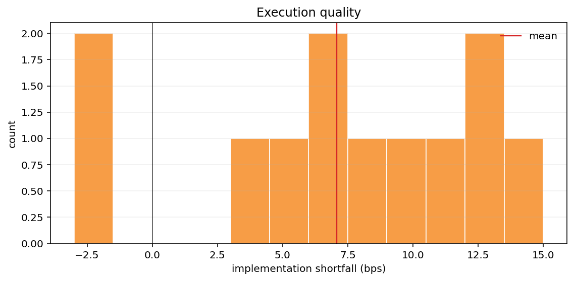
execution_fig = fp.plot_execution_quality(execution_quality)

Post-Trade Tables

cost_table = fp.table_cost_breakdown(cost_breakdown)
round_trip_table = fp.table_round_trip_stats(round_trips)
execution_table = fp.table_execution_quality(execution_quality)

Component	Total	Pct total
commission	5.00	25.15%
fees	1.25	6.29%
slippage	13.63	68.56%

Metric	Value
Trades	3.00
Win rate	66.67%
Average PnL	160.00
Total PnL	480.00
Profit factor	3.00
Payoff ratio	1.50

Metric	Value
Count	12
Mean bps	7.08
Median bps	7.50
Worst bps	15.00
Best bps	-3.00

Alpha IC Plots

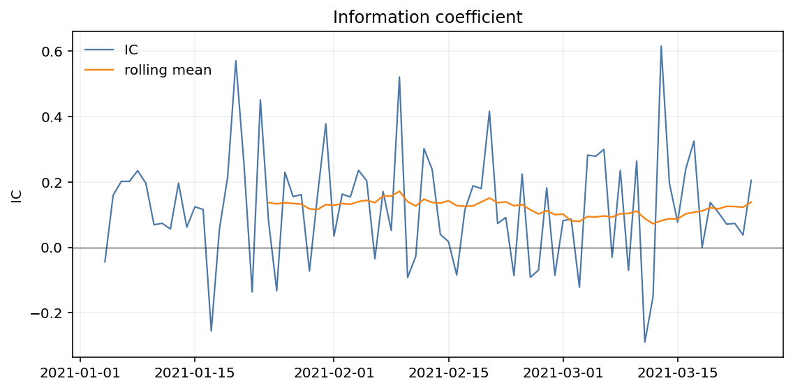
ic_ts_fig = fp.plot_ic_ts(ic)
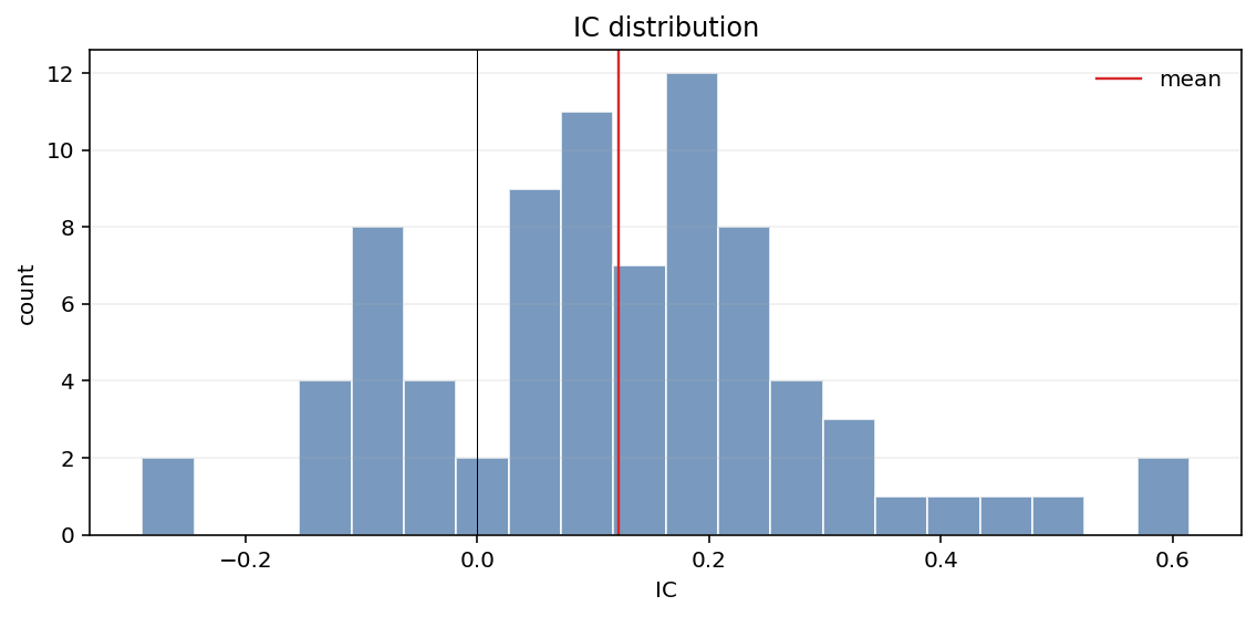
ic_hist_fig = fp.plot_ic_hist(ic)
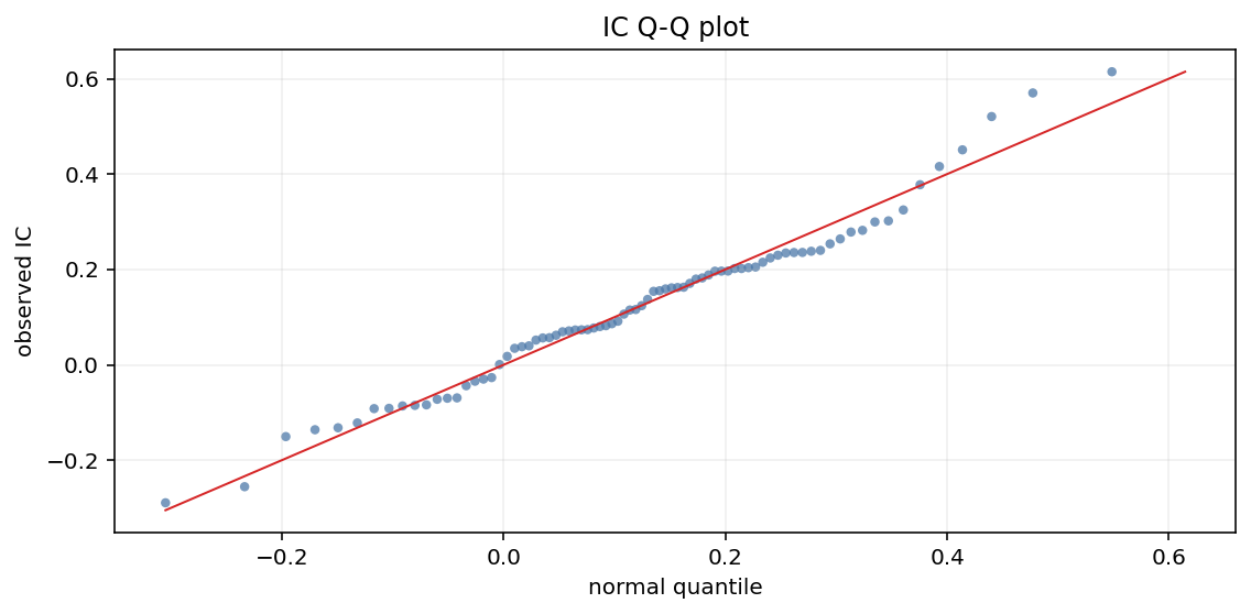
ic_qq_fig = fp.plot_ic_qq(ic)
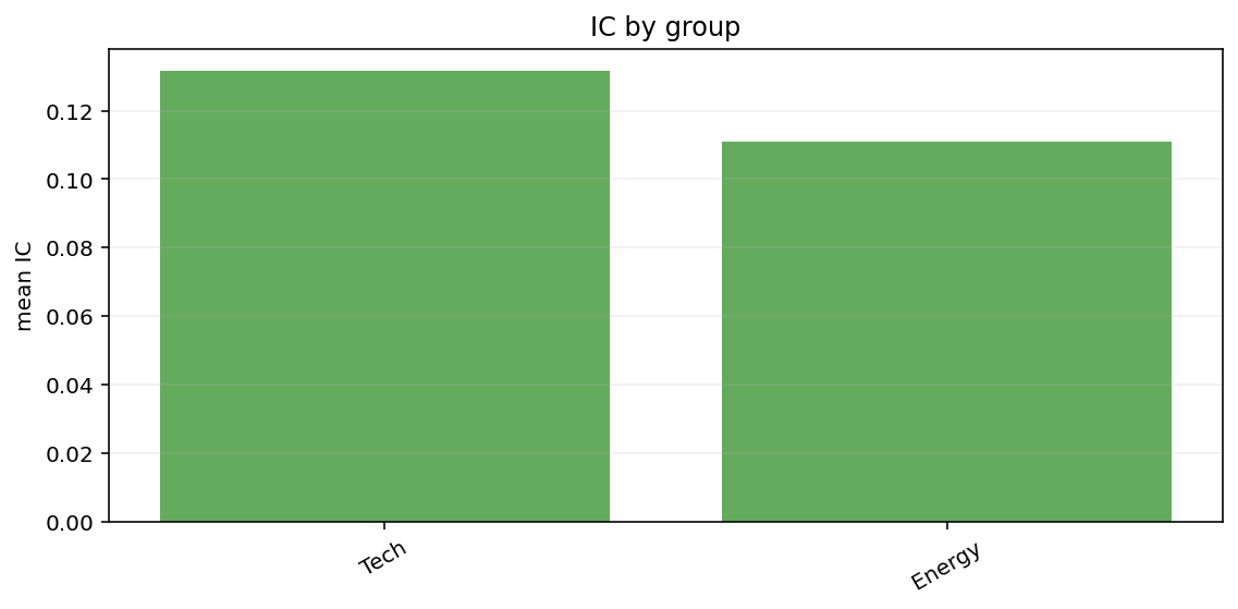
ic_group_fig = fp.plot_ic_by_group(ic_by_group.to_pandas())
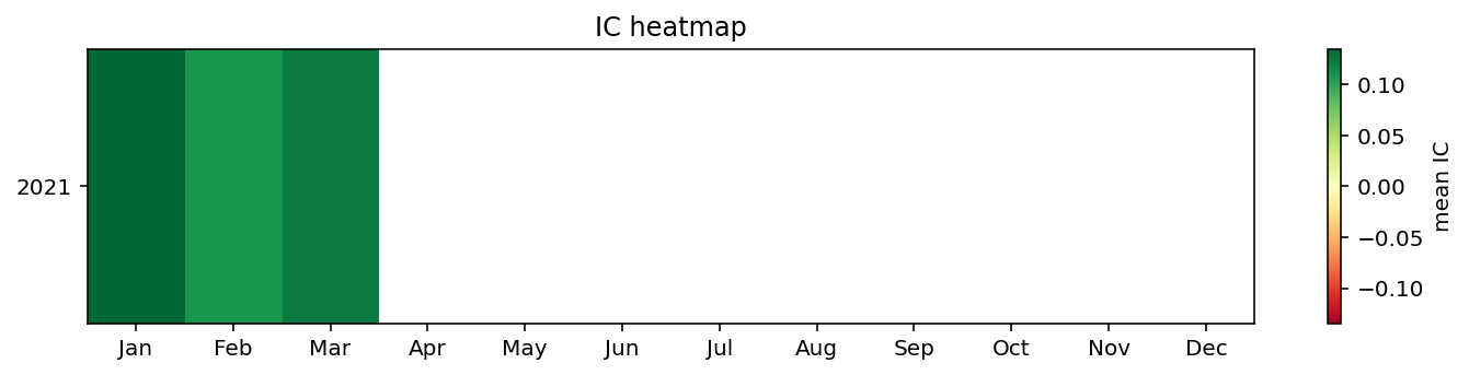
ic_heatmap_fig = fp.plot_ic_heatmap(ic, period="month")
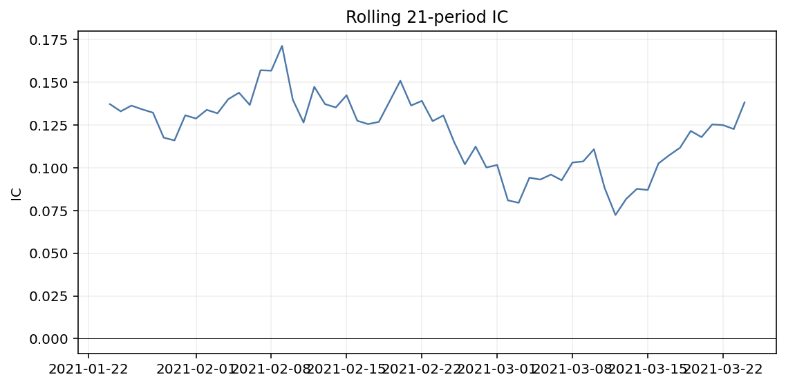
rolling_ic_fig = fp.plot_rolling_ic(ic, window=21)

Alpha Quantile Plots

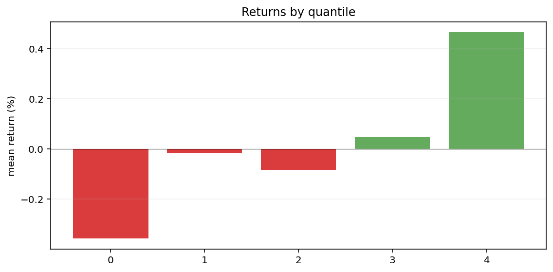
quantile_bar_fig = fp.plot_quantile_returns_bar(alpha_frame)
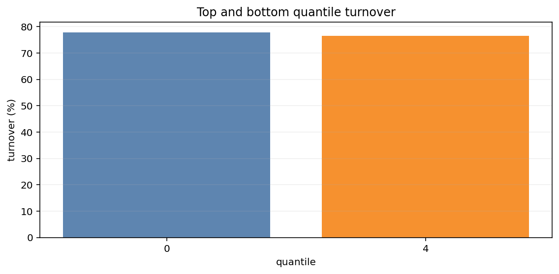
turnover_fig = fp.plot_top_bottom_quantile_turnover(alpha_frame)
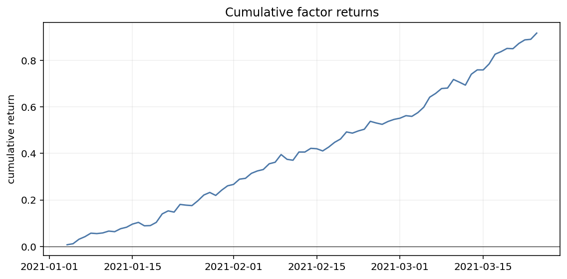
factor_return_fig = fp.plot_cumulative_factor_returns(factor_returns)

Alpha Analysis Tables

information_table = fp.table_information(ic)
quantile_return_table = fp.table_returns_by_quantile(alpha_frame)
turnover_table = fp.table_turnover(alpha_frame)
quantile_stats_table = fp.table_quantile_statistics(alpha_frame)

Metric	Value
Mean IC	0.12
IC volatility	0.17
ICIR	0.71
t-stat	6.38
Positive IC	77.50%
Observations	80

Quantile	Count	Mean return	Volatility
0	80	-0.36%	0.75%
1	80	-0.02%	0.70%
2	80	-0.08%	0.74%
3	80	0.05%	0.70%
4	80	0.47%	0.65%

Quantile	Turnover
0	77.81%
1	78.12%
2	78.28%
3	78.59%
4	76.56%

Quantile	Count	Signal mean	Signal std
0	640	-1.40	0.21
1	640	-0.53	0.19
2	640	0.01	0.18
3	640	0.53	0.16
4	640	1.38	0.24

---

Generate Every Example Artifact

Use the packaged helper when you want all examples written to disk:

from finance_plots.gallery import generate_gallery

outputs = generate_gallery("docs/assets/gallery")